相关知识

Diffusion扩散模型

这是一类生成模型，用于生成高质量的数据样本如图像、音频等。基本思想是通过模拟数据从噪声逐步变为目标数据的过程，来生成新的数据样本。diffusion对图像的处理包括

• 预定义的正向扩散过程q，将高斯噪声添加到图像中，最终得到纯噪声
• 学习的反向去噪的扩散过程：训练神经网络从噪声开始逐渐去噪，最终得到实际图像
  由 $t$ 索引的正向和反向过程都发生在某些有限时间步长 $T$（DDPM作者使用 $T=1000$）内。从$t=0$开始，在数据分布中采样真实图像 ${\mathbf{x}}_0$，正向过程在每个时间步长 $t$ 都从高斯分布中采样一些噪声，再添加到上一个时刻的图像中。
  假定给定一个足够大的 $T$ 和一个在每个时间步长添加噪声的良好时间表，
  最终会在 $t=T$ 通过渐进的过程得到所谓的[各向同性的高斯分布]

实现原理

前向过程

这里就是给图片加噪声的过程。前向过程中每个时刻t只和时刻t-1有关。而随着时间步的增大，图像xt就越来越接近纯高斯噪声。
那么，如果我们知道条件概率分布 $p({\mathbf{x}}_{t-1}|{\mathbf{x}}_t)$ ，我们就可以反向运行这个过程：通过采样一些随机高斯噪声 ${\mathbf{x}}_T$，然后逐渐去噪它，最终得到真实分布 ${\mathbf{x}}_0$ 中的样本。但是，我们不知道条件概率分布 $p({\mathbf{x}}_{t-1}|{\mathbf{x}}_t)$ 。这很棘手，因为需要知道所有可能图像的分布，才能计算这个条件概率。

逆向过程

为了解决上述问题，我们将利用神经网络来近似（学习）这个条件概率分布 $p_{\theta }({\mathbf{x}}_{t-1}|{\mathbf{x}}_t)$ , 其中 $\theta$ 是神经网络的参数。前向是加噪的过程，逆向是去噪推理过程，而通过神经网络学习并表示 $p_{\theta }({\mathbf{x}}_{t-1}|{\mathbf{x}}_t)$ 的过程就是Diffusion 逆向去噪的核心。

现在，我们知道了需要一个神经网络来学习逆向过程的（条件）概率分布。我们假设这个反向过程也是高斯的，任何高斯分布都由2个参数定义：

• 由 ${\mu }_{\theta }$ 参数化的平均值

• 由 ${\mu }_{\theta }$ 参数化的方差

平均值和方差也取决于噪声水平 $t$ ，神经网络需要通过学习来表示这些均值和方差。

• 注意，DDPM的作者决定保持方差固定，让神经网络只学习（表示）这个条件概率分布的平均值 ${\mu }_{\theta }$ 。

为了导出一个目标函数来学习反向过程的平均值，作者观察到 $q$ 和 $p_{\theta }$ 的组合可以被视为变分自动编码器(VAE)。因此，变分下界（也称为ELBO）可用于最小化真值数据样本 ${\mathbf{x}}_0$ 的似然负对数（有关ELBO的详细信息，请参阅VAE论文（Kingma等人，2013年）），该过程的ELBO是每个时间步长的损失之和 $L=L_0+L_1+...+L_T$ ，其中，每项的损失 $L_t$ （除了 $L_0$ ）实际上是2个高斯分布之间的KL发散，可以明确地写为相对于均值的L2-loss!

如Sohl-Dickstein等人所示，构建Diffusion正向过程的直接结果是我们可以在条件是 ${\mathbf{x}}_0$ （因为高斯和也是高斯）的情况下，在任意噪声水平上采样 ${\mathbf{x}}_t$ ，而不需要重复应用 $q$ 去采样 ${\mathbf{x}}_t$ ，这非常方便。使用

$$\begin{gathered} {\alpha }_t:=1-{\beta }_t \\ \bar{\alpha }t:={\Pi }_{s=1}^t{\alpha }_s \end{gathered}$$

我们就有

$$q({\mathbf{x}}_t|{\mathbf{x}}_0)=\mathcal{N}({\mathbf{x}}_t;\sqrt{{\bar{\alpha }}_t}{\mathbf{x}}_0,(1-{\bar{\alpha }}_t)\mathbf{I})$$

这意味着我们可以采样高斯噪声并适当地缩放它，然后将其添加到 ${\mathbf{x}}_0$ 中，直接获得 ${\mathbf{x}}_t$ 。

请注意，${\bar{\alpha }}_t$ 是已知 ${\beta }_t$ 方差计划的函数，因此也是已知的，可以预先计算。这允许我们在训练期间优化损失函数 $L$ 的随机项。或者换句话说，在训练期间随机采样 $t$ 并优化 $L_t$ 。

正如Ho等人所展示的那样，这种性质的另一个优点是可以重新参数化平均值，使神经网络学习（预测）构成损失的KL项中噪声的附加噪声。这意味着我们的神经网络变成了噪声预测器，而不是（直接）均值预测器。其中，平均值可以按如下方式计算：

$${\mu }_{\theta }({\mathbf{x}}_t,t)=\frac{1}{\sqrt{{\alpha }_t}}\left({\mathbf{x}}_t-\frac{{\beta }_t}{\sqrt{1-{\bar{\alpha }}_t}}{ϵ}_{\theta }({\mathbf{x}}_t,t)\right)$$

最终的目标函数 $L_t$ 如下 （随机步长 t 由 $(ϵ\sim N(0,\mathbf{I}))$ 给定）：

$$\Vert ϵ-{ϵ}_{\theta }({\mathbf{x}}_t,t){\Vert }^2=\Vert ϵ-{ϵ}_{\theta }(\sqrt{{\bar{\alpha }}_t}{\mathbf{x}}_0+\sqrt{(1-{\bar{\alpha }}_t)}ϵ,t){\Vert }^2$$

在这里， ${\mathbf{x}}_0$ 是初始（真实，未损坏）图像， $ϵ$ 是在时间步长 $t$ 采样的纯噪声，${ϵ}_{\theta }({\mathbf{x}}_t,t)$是我们的神经网络。神经网络是基于真实噪声和预测高斯噪声之间的简单均方误差（MSE）进行优化的。

训练算法现在如下所示：

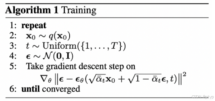
换句话说：

• 我们从真实未知和可能复杂的数据分布中随机抽取一个样本 $q({\mathbf{x}}_0)$

• 我们均匀地采样$1$和$T$之间的噪声水平$t$（即，随机时间步长）

• 我们从高斯分布中采样一些噪声，并使用上面定义的属性在 $t$ 时间步上破坏输入

• 神经网络被训练以基于损坏的图像 ${\mathbf{x}}_t$ 来预测这种噪声，即基于已知的时间表 ${\mathbf{x}}_t$ 上施加的噪声

实际上，所有这些都是在批数据上使用随机梯度下降来优化神经网络完成的。

U-Net神经网络预测噪声

神经网络需要在特定时间步长接收带噪声的图像，并返回预测的噪声。请注意，预测噪声是与输入图像具有相同大小/分辨率的张量。因此，从技术上讲，网络接受并输出相同形状的张量。那么我们可以用什么类型的神经网络来实现呢？

这里通常使用的是非常相似的自动编码器，您可能还记得典型的"深度学习入门"教程。自动编码器在编码器和解码器之间有一个所谓的"bottleneck"层。编码器首先将图像编码为一个称为"bottleneck"的较小的隐藏表示，然后解码器将该隐藏表示解码回实际图像。这迫使网络只保留bottleneck层中最重要的信息。

在模型结构方面，DDPM的作者选择了U-Net，出自（Ronneberger et al.，2015）（当时，它在医学图像分割方面取得了最先进的结果）。这个网络就像任何自动编码器一样，在中间由一个bottleneck组成，确保网络只学习最重要的信息。重要的是，它在编码器和解码器之间引入了残差连接，极大地改善了梯度流（灵感来自于（He et al., 2015））。

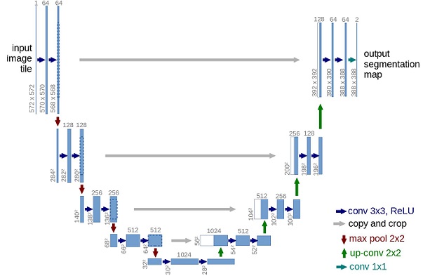
可以看出，U-Net模型首先对输入进行下采样（即，在空间分辨率方面使输入更小），之后执行上采样。

实验

工具函数定义

def rearrange(head, inputs):
    b, hc, x, y = inputs.shape
    c = hc // head
    return inputs.reshape((b, head, c, x * y))

def rsqrt(x):
    res = ops.sqrt(x)
    return ops.inv(res)

def randn_like(x, dtype=None):
    if dtype is None:
        dtype = x.dtype
    res = ops.standard_normal(x.shape).astype(dtype)
    return res

def randn(shape, dtype=None):
    if dtype is None:
        dtype = ms.float32
    res = ops.standard_normal(shape).astype(dtype)
    return res

def randint(low, high, size, dtype=ms.int32):
    res = ops.uniform(size, Tensor(low, dtype), Tensor(high, dtype), dtype=dtype)
    return res

def exists(x):
    return x is not None

def default(val, d):
    if exists(val):
        return val
    return d() if callable(d) else d

def _check_dtype(d1, d2):
    if ms.float32 in (d1, d2):
        return ms.float32
    if d1 == d2:
        return d1
    raise ValueError('dtype is not supported.')

class Residual(nn.Cell):
    def __init__(self, fn):
        super().__init__()
        self.fn = fn

    def construct(self, x, *args, **kwargs):
        return self.fn(x, *args, **kwargs) + x
# 定义上下采样操作的别名
def Upsample(dim):
    return nn.Conv2dTranspose(dim, dim, 4, 2, pad_mode="pad", padding=1)

def Downsample(dim):
    return nn.Conv2d(dim, dim, 4, 2, pad_mode="pad", padding=1)

位置向量

使用正弦位置嵌入来编码t，对于批处理中的每一张图像，神经网络"知道"它在哪个特定时间步长（噪声水平）上运行。SinusoidalPositionEmbeddings模块采用(batch_size, 1)形状的张量作为输入（即批处理中几个有噪声图像的噪声水平），并将其转换为(batch_size, dim)形状的张量，其中dim是位置嵌入的尺寸。然后，我们将其添加到每个剩余块中。

class SinusoidalPositionEmbeddings(nn.Cell):
    def __init__(self, dim):
        super().__init__()
        self.dim = dim
        half_dim = self.dim // 2
        emb = math.log(10000) / (half_dim - 1)
        emb = np.exp(np.arange(half_dim) * - emb)
        self.emb = Tensor(emb, ms.float32)

    def construct(self, x):
        emb = x[:, None] * self.emb[None, :]
        emb = ops.concat((ops.sin(emb), ops.cos(emb)), axis=-1)
        return emb

ResNet/ConvNeXT块

这是U-Net模型的核心构建块。这里使用ConNeXT构建。

class Block(nn.Cell):
    def __init__(self, dim, dim_out, groups=1):
        super().__init__()
        self.proj = nn.Conv2d(dim, dim_out, 3, pad_mode="pad", padding=1)
        self.proj = c(dim, dim_out, 3, padding=1, pad_mode='pad')
        self.norm = nn.GroupNorm(groups, dim_out)
        self.act = nn.SiLU()

    def construct(self, x, scale_shift=None):
        x = self.proj(x)
        x = self.norm(x)

        if exists(scale_shift):
            scale, shift = scale_shift
            x = x * (scale + 1) + shift

        x = self.act(x)
        return x

class ConvNextBlock(nn.Cell):
    def __init__(self, dim, dim_out, *, time_emb_dim=None, mult=2, norm=True):
        super().__init__()
        self.mlp = (
            nn.SequentialCell(nn.GELU(), nn.Dense(time_emb_dim, dim))
            if exists(time_emb_dim)
            else None
        )

        self.ds_conv = nn.Conv2d(dim, dim, 7, padding=3, group=dim, pad_mode="pad")
        self.net = nn.SequentialCell(
            nn.GroupNorm(1, dim) if norm else nn.Identity(),
            nn.Conv2d(dim, dim_out * mult, 3, padding=1, pad_mode="pad"),
            nn.GELU(),
            nn.GroupNorm(1, dim_out * mult),
            nn.Conv2d(dim_out * mult, dim_out, 3, padding=1, pad_mode="pad"),
        )

        self.res_conv = nn.Conv2d(dim, dim_out, 1) if dim != dim_out else nn.Identity()

    def construct(self, x, time_emb=None):
        h = self.ds_conv(x)
        if exists(self.mlp) and exists(time_emb):
            assert exists(time_emb), "time embedding must be passed in"
            condition = self.mlp(time_emb)
            condition = condition.expand_dims(-1).expand_dims(-1)
            h = h + condition

        h = self.net(h)
        return h + self.res_conv(x)

Attention模块

这里使用Transformer架构的SiLU，DDPM将其加入到卷积块之间。Phil Wang使用了两种注意力变体：一种是常规的multi-head self-attention（如Transformer中使用的），另一种是LinearAttention(Shen et al., 2018)，其时间和内存要求在序列长度上线性缩放，而不是在常规注意力中缩放。

class Attention(nn.Cell):
    def __init__(self, dim, heads=4, dim_head=32):
        super().__init__()
        self.scale = dim_head ** -0.5
        self.heads = heads
        hidden_dim = dim_head * heads

        self.to_qkv = nn.Conv2d(dim, hidden_dim * 3, 1, pad_mode='valid', has_bias=False)
        self.to_out = nn.Conv2d(hidden_dim, dim, 1, pad_mode='valid', has_bias=True)
        self.map = ops.Map()
        self.partial = ops.Partial()

    def construct(self, x):
        b, _, h, w = x.shape
        qkv = self.to_qkv(x).chunk(3, 1)
        q, k, v = self.map(self.partial(rearrange, self.heads), qkv)

        q = q * self.scale

        # 'b h d i, b h d j -> b h i j'
        sim = ops.bmm(q.swapaxes(2, 3), k)
        attn = ops.softmax(sim, axis=-1)
        # 'b h i j, b h d j -> b h i d'
        out = ops.bmm(attn, v.swapaxes(2, 3))
        out = out.swapaxes(-1, -2).reshape((b, -1, h, w))

        return self.to_out(out)


class LayerNorm(nn.Cell):
    def __init__(self, dim):
        super().__init__()
        self.g = Parameter(initializer('ones', (1, dim, 1, 1)), name='g')

    def construct(self, x):
        eps = 1e-5
        var = x.var(1, keepdims=True)
        mean = x.mean(1, keep_dims=True)
        return (x - mean) * rsqrt((var + eps)) * self.g


class LinearAttention(nn.Cell):
    def __init__(self, dim, heads=4, dim_head=32):
        super().__init__()
        self.scale = dim_head ** -0.5
        self.heads = heads
        hidden_dim = dim_head * heads
        self.to_qkv = nn.Conv2d(dim, hidden_dim * 3, 1, pad_mode='valid', has_bias=False)

        self.to_out = nn.SequentialCell(
            nn.Conv2d(hidden_dim, dim, 1, pad_mode='valid', has_bias=True),
            LayerNorm(dim)
        )

        self.map = ops.Map()
        self.partial = ops.Partial()

    def construct(self, x):
        b, _, h, w = x.shape
        qkv = self.to_qkv(x).chunk(3, 1)
        q, k, v = self.map(self.partial(rearrange, self.heads), qkv)

        q = ops.softmax(q, -2)
        k = ops.softmax(k, -1)

        q = q * self.scale
        v = v / (h * w)

        # 'b h d n, b h e n -> b h d e'
        context = ops.bmm(k, v.swapaxes(2, 3))
        # 'b h d e, b h d n -> b h e n'
        out = ops.bmm(context.swapaxes(2, 3), q)

        out = out.reshape((b, -1, h, w))
        return self.to_out(out)

组归一化

DDPM作者将U-Net的卷积/注意层与群归一化。这里定义PreNorm类用于在注意层之前应用groupnorm。

class PreNorm(nn.Cell):
    def __init__(self, dim, fn):
        super().__init__()
        self.fn = fn
        self.norm = nn.GroupNorm(1, dim)

    def construct(self, x):
        x = self.norm(x)
        return self.fn(x)

条件U-Net

我们已经定义了所有的构建块（位置嵌入、ResNet/ConvNeXT块、Attention和组归一化），现在需要定义整个神经网络了。请记住，网络 ${ϵ}_{\theta }({\mathbf{x}}_t,t)$ 的工作是接收一批噪声图像+噪声水平，并输出添加到输入中的噪声。

更具体的：
网络获取了一批(batch_size, num_channels, height, width)形状的噪声图像和一批(batch_size, 1)形状的噪音水平作为输入，并返回(batch_size, num_channels, height, width)形状的张量。

网络构建过程如下：

• 首先，将卷积层应用于噪声图像批上，并计算噪声水平的位置

• 接下来，应用一系列下采样级。每个下采样阶段由2个ResNet/ConvNeXT块 + groupnorm + attention + 残差连接 + 一个下采样操作组成

• 在网络的中间，再次应用ResNet或ConvNeXT块，并与attention交织

• 接下来，应用一系列上采样级。每个上采样级由2个ResNet/ConvNeXT块+ groupnorm + attention + 残差连接 + 一个上采样操作组成

• 最后，应用ResNet/ConvNeXT块，然后应用卷积层

最终，神经网络将层堆叠完成搭建。

class Unet(nn.Cell):
    def __init__(
            self,
            dim,
            init_dim=None,
            out_dim=None,
            dim_mults=(1, 2, 4, 8),
            channels=3,
            with_time_emb=True,
            convnext_mult=2,
    ):
        super().__init__()

        self.channels = channels

        init_dim = default(init_dim, dim // 3 * 2)
        self.init_conv = nn.Conv2d(channels, init_dim, 7, padding=3, pad_mode="pad", has_bias=True)

        dims = [init_dim, *map(lambda m: dim * m, dim_mults)]
        in_out = list(zip(dims[:-1], dims[1:]))

        block_klass = partial(ConvNextBlock, mult=convnext_mult)

        if with_time_emb:
            time_dim = dim * 4
            self.time_mlp = nn.SequentialCell(
                SinusoidalPositionEmbeddings(dim),
                nn.Dense(dim, time_dim),
                nn.GELU(),
                nn.Dense(time_dim, time_dim),
            )
        else:
            time_dim = None
            self.time_mlp = None

        self.downs = nn.CellList([])
        self.ups = nn.CellList([])
        num_resolutions = len(in_out)

        for ind, (dim_in, dim_out) in enumerate(in_out):
            is_last = ind >= (num_resolutions - 1)

            self.downs.append(
                nn.CellList(
                    [
                        block_klass(dim_in, dim_out, time_emb_dim=time_dim),
                        block_klass(dim_out, dim_out, time_emb_dim=time_dim),
                        Residual(PreNorm(dim_out, LinearAttention(dim_out))),
                        Downsample(dim_out) if not is_last else nn.Identity(),
                    ]
                )
            )

        mid_dim = dims[-1]
        self.mid_block1 = block_klass(mid_dim, mid_dim, time_emb_dim=time_dim)
        self.mid_attn = Residual(PreNorm(mid_dim, Attention(mid_dim)))
        self.mid_block2 = block_klass(mid_dim, mid_dim, time_emb_dim=time_dim)

        for ind, (dim_in, dim_out) in enumerate(reversed(in_out[1:])):
            is_last = ind >= (num_resolutions - 1)

            self.ups.append(
                nn.CellList(
                    [
                        block_klass(dim_out * 2, dim_in, time_emb_dim=time_dim),
                        block_klass(dim_in, dim_in, time_emb_dim=time_dim),
                        Residual(PreNorm(dim_in, LinearAttention(dim_in))),
                        Upsample(dim_in) if not is_last else nn.Identity(),
                    ]
                )
            )

        out_dim = default(out_dim, channels)
        self.final_conv = nn.SequentialCell(
            block_klass(dim, dim), nn.Conv2d(dim, out_dim, 1)
        )

    def construct(self, x, time):
        x = self.init_conv(x)

        t = self.time_mlp(time) if exists(self.time_mlp) else None

        h = []

        for block1, block2, attn, downsample in self.downs:
            x = block1(x, t)
            x = block2(x, t)
            x = attn(x)
            h.append(x)

            x = downsample(x)

        x = self.mid_block1(x, t)
        x = self.mid_attn(x)
        x = self.mid_block2(x, t)

        len_h = len(h) - 1
        for block1, block2, attn, upsample in self.ups:
            x = ops.concat((x, h[len_h]), 1)
            len_h -= 1
            x = block1(x, t)
            x = block2(x, t)
            x = attn(x)

            x = upsample(x)
        return self.final_conv(x)

正向扩散

使用线性时间表，将正向过程方差设置为常数，从${\beta }_1=10^{-4}$线性增加到${\beta }_T=0.02$。

def linear_beta_schedule(timesteps):
    beta_start = 0.0001
    beta_end = 0.02
    return np.linspace(beta_start, beta_end, timesteps).astype(np.float32)

# 扩散200步
timesteps = 200

# 定义 beta schedule
betas = linear_beta_schedule(timesteps=timesteps)

# 定义 alphas
alphas = 1. - betas
alphas_cumprod = np.cumprod(alphas, axis=0)
alphas_cumprod_prev = np.pad(alphas_cumprod[:-1], (1, 0), constant_values=1)

sqrt_recip_alphas = Tensor(np.sqrt(1. / alphas))
sqrt_alphas_cumprod = Tensor(np.sqrt(alphas_cumprod))
sqrt_one_minus_alphas_cumprod = Tensor(np.sqrt(1. - alphas_cumprod))

# 计算 q(x_{t-1} | x_t, x_0)
posterior_variance = betas * (1. - alphas_cumprod_prev) / (1. - alphas_cumprod)

p2_loss_weight = (1 + alphas_cumprod / (1 - alphas_cumprod)) ** -0.
p2_loss_weight = Tensor(p2_loss_weight)

def extract(a, t, x_shape):
    b = t.shape[0]
    out = Tensor(a).gather(t, -1)
    return out.reshape(b, *((1,) * (len(x_shape) - 1)))

接下来添加噪音，首先通过除以$255$来标准化图像（使它们在 $[0,1]$ 范围内），然后确保它们在 $[-1,1]$ 范围内。

image_size = 128
transforms = [
    Resize(image_size, Inter.BILINEAR),
    CenterCrop(image_size),
    ToTensor(),
    lambda t: (t * 2) - 1
]


path = './image_cat'
dataset = ImageFolderDataset(dataset_dir=path, num_parallel_workers=cpu_count(),
                             extensions=['.jpg', '.jpeg', '.png', '.tiff'],
                             num_shards=1, shard_id=0, shuffle=False, decode=True)
dataset = dataset.project('image')
transforms.insert(1, RandomHorizontalFlip())
dataset_1 = dataset.map(transforms, 'image')
dataset_2 = dataset_1.batch(1, drop_remainder=True)
x_start = next(dataset_2.create_tuple_iterator())[0]
print(x_start.shape)
# (1, 3, 128, 128)

定义反向变换，接收包含[-1,1]中的张量，并将它们转回PIL图像。

reverse_transform = [
    lambda t: (t + 1) / 2,
    lambda t: ops.permute(t, (1, 2, 0)), # CHW to HWC
    lambda t: t * 255.,
    lambda t: t.asnumpy().astype(np.uint8),
    ToPIL()
]

def compose(transform, x):
    for d in transform:
        x = d(x)
    return x

定义前向扩散过程

def q_sample(x_start, t, noise=None):
    if noise is None:
        noise = randn_like(x_start)
    return (extract(sqrt_alphas_cumprod, t, x_start.shape) * x_start +
            extract(sqrt_one_minus_alphas_cumprod, t, x_start.shape) * noise)

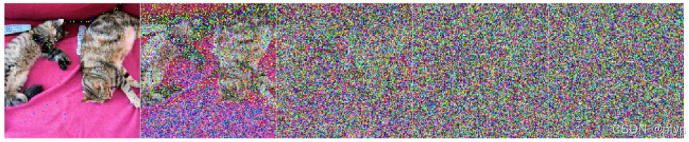
可视化一下噪声增加的过程

def plot(imgs, with_orig=False, row_title=None, **imshow_kwargs):
    if not isinstance(imgs[0], list):
        imgs = [imgs]

    num_rows = len(imgs)
    num_cols = len(imgs[0]) + with_orig
    _, axs = plt.subplots(figsize=(200, 200), nrows=num_rows, ncols=num_cols, squeeze=False)
    for row_idx, row in enumerate(imgs):
        row = [image] + row if with_orig else row
        for col_idx, img in enumerate(row):
            ax = axs[row_idx, col_idx]
            ax.imshow(np.asarray(img), **imshow_kwargs)
            ax.set(xticklabels=[], yticklabels=[], xticks=[], yticks=[])

    if with_orig:
        axs[0, 0].set(title='Original image')
        axs[0, 0].title.set_size(8)
    if row_title is not None:
        for row_idx in range(num_rows):
            axs[row_idx, 0].set(ylabel=row_title[row_idx])

    plt.tight_layout()

定义损失函数

def p_losses(unet_model, x_start, t, noise=None):
    if noise is None:
        noise = randn_like(x_start)
    x_noisy = q_sample(x_start=x_start, t=t, noise=noise)
    predicted_noise = unet_model(x_noisy, t)

    loss = nn.SmoothL1Loss()(noise, predicted_noise)# todo
    loss = loss.reshape(loss.shape[0], -1)
    loss = loss * extract(p2_loss_weight, t, loss.shape)
    return loss.mean()

数据处理

定义一个正则数据集。数据集可以来自简单的真实数据集的图像组成，如Fashion-MNIST、CIFAR-10或ImageNet，其中线性缩放为 $[-1,1]$ 。

每个图像的大小都会调整为相同的大小。有趣的是，图像也是随机水平翻转的。根据论文内容：我们在CIFAR10的训练中使用了随机水平翻转；我们尝试了有翻转和没有翻转的训练，并发现翻转可以稍微提高样本质量。

本实验我们选用Fashion_MNIST数据集，此数据集由已经具有相同分辨率的图像组成，即28x28。

image_size = 28
channels = 1
batch_size = 2

fashion_mnist_dataset_dir = "./dataset"
dataset = FashionMnistDataset(dataset_dir=fashion_mnist_dataset_dir, usage="train", 
                              num_parallel_workers=cpu_count(), shuffle=True,
                              num_shards=1, shard_id=0, num_samples=4000)
# 随机水平翻转、使值在[-1,1]中
transforms = [
    RandomHorizontalFlip(),
    ToTensor(),
    lambda t: (t * 2) - 1
]


dataset = dataset.project('image')
dataset = dataset.shuffle(64)
dataset = dataset.map(transforms, 'image')
dataset = dataset.batch(2, drop_remainder=True)

采样

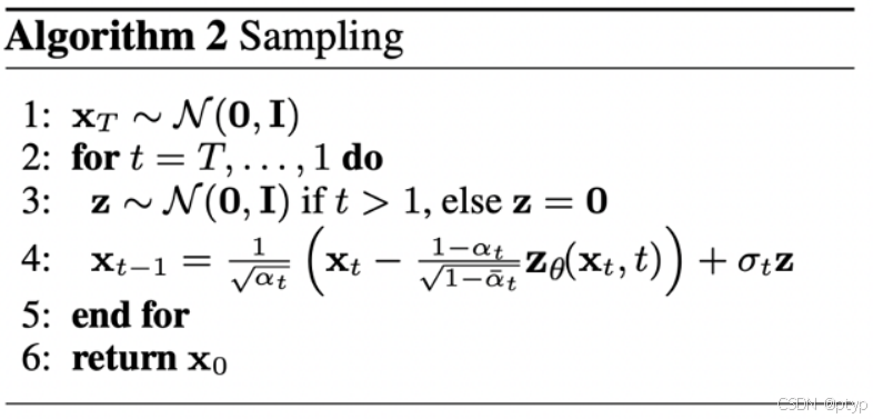
这一步是为了追踪模型进度。从扩散模型生成新图像是通过反转扩散过程来实现的：我们从$T$开始，我们从高斯分布中采样纯噪声，然后使用我们的神经网络逐渐去噪（使用它所学习的条件概率），直到我们最终在时间步$t=0$结束。如上图所示，我们可以通过使用我们的噪声预测器插入平均值的重新参数化，导出一个降噪程度较低的图像
${\mathbf{x}}_{t-1}$。请注意，方差是提前知道的。

理想情况下，我们最终会得到一个看起来像是来自真实数据分布的图像。

def p_sample(model, x, t, t_index):
    betas_t = extract(betas, t, x.shape)
    sqrt_one_minus_alphas_cumprod_t = extract(
        sqrt_one_minus_alphas_cumprod, t, x.shape
    )
    sqrt_recip_alphas_t = extract(sqrt_recip_alphas, t, x.shape)
    model_mean = sqrt_recip_alphas_t * (x - betas_t * model(x, t) / sqrt_one_minus_alphas_cumprod_t)

    if t_index == 0:
        return model_mean
    posterior_variance_t = extract(posterior_variance, t, x.shape)
    noise = randn_like(x)
    return model_mean + ops.sqrt(posterior_variance_t) * noise

def p_sample_loop(model, shape):
    b = shape[0]
    # 从纯噪声开始
    img = randn(shape, dtype=None)
    imgs = []

    for i in tqdm(reversed(range(0, timesteps)), desc='sampling loop time step', total=timesteps):
        img = p_sample(model, img, ms.numpy.full((b,), i, dtype=mstype.int32), i)
        imgs.append(img.asnumpy())
    return imgs

def sample(model, image_size, batch_size=16, channels=3):
    return p_sample_loop(model, shape=(batch_size, channels, image_size, image_size))

训练

# 定义动态学习率
lr = nn.cosine_decay_lr(min_lr=1e-7, max_lr=1e-4, total_step=1*2000, step_per_epoch=2000, decay_epoch=1)

# 定义 Unet模型
unet_model = Unet(
    dim=image_size,
    channels=channels,
    dim_mults=(1, 2, 4,)
)

name_list = []
for (name, par) in list(unet_model.parameters_and_names()):
    name_list.append(name)
i = 0
for item in list(unet_model.trainable_params()):
    item.name = name_list[i]
    i += 1

# 定义优化器
optimizer = nn.Adam(unet_model.trainable_params(), learning_rate=lr)
loss_scaler = DynamicLossScaler(65536, 2, 1000)

# 定义前向过程
def forward_fn(data, t, noise=None):
    loss = p_losses(unet_model, data, t, noise)
    return loss

# 计算梯度
grad_fn = ms.value_and_grad(forward_fn, None, optimizer.parameters, has_aux=False)

# 梯度更新
def train_step(data, t, noise):
    loss, grads = grad_fn(data, t, noise)
    optimizer(grads)
    return loss

import time

# 由于时间问题和内存问题，在 CPU 环境下 epoch 设置为 1，可以根据需求进行调整。建议在 Ascend/GPU 环境体验该教程。
epochs = 1

for epoch in range(epochs):
    begin_time = time.time()
    for step, batch in enumerate(dataset.create_tuple_iterator()):
        unet_model.set_train()
        batch_size = batch[0].shape[0]
        t = randint(0, timesteps, (batch_size,), dtype=ms.int32)
        noise = randn_like(batch[0])
        loss = train_step(batch[0], t, noise)

        if step % 100 == 0:
            print(" epoch: ", epoch, " step: ", step, " Loss: ", loss)
    end_time = time.time()
    times = end_time - begin_time
    print("training time:", times, "s")
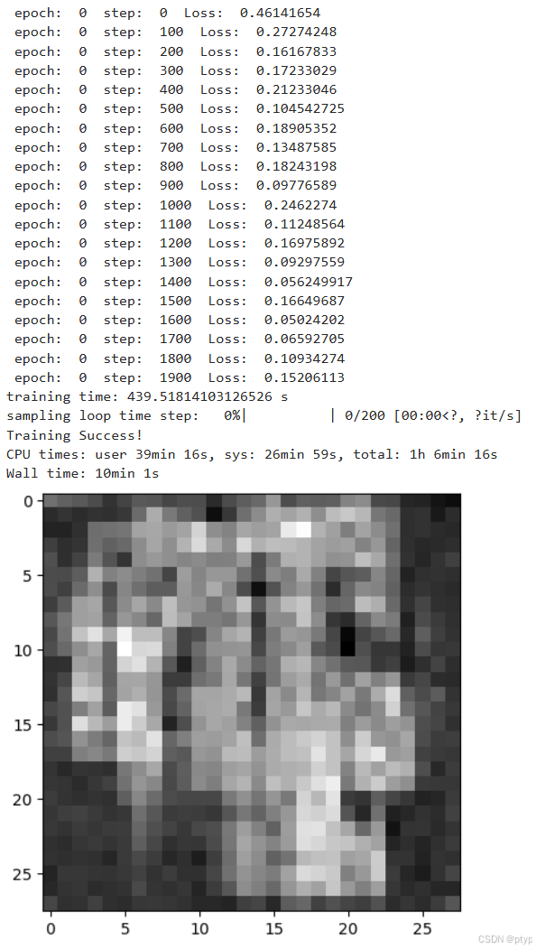
# 展示随机采样效果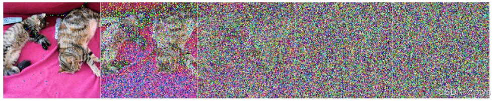![在这里插入图片描述](https://i-blog.csdnimg.cn/direct/aa4d0a5fb2334e5c8456076ff167824e.png)

unet_model.set_train(False)
samples = sample(unet_model, image_size=image_size, batch_size=64, channels=channels)
plt.imshow(samples[-1][5].reshape(image_size, image_size, channels), cmap="gray")
print("Training Success!")

训练效果如下

推理/从模型中采样

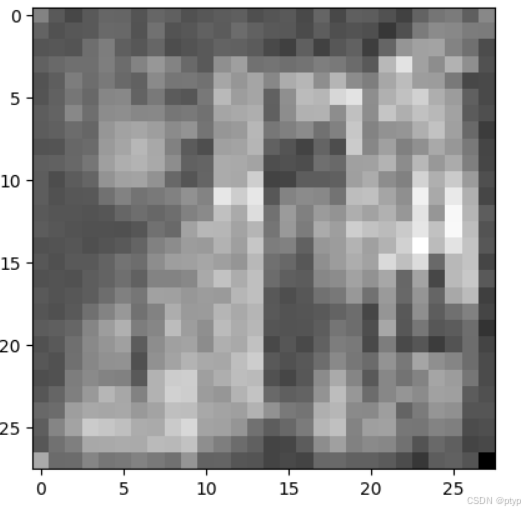
使用上面定义的采样函数展示一个随机效果

# 采样64个图片
unet_model.set_train(False)
samples = sample(unet_model, image_size=image_size, batch_size=64, channels=channels)
# 展示一个随机效果
random_index = 5
plt.imshow(samples[-1][random_index].reshape(image_size, image_size, channels), cmap="gray")

后续工作（2022年之前）

改进的去噪扩散概率模型(Nichol et al., 2021)：发现学习条件分布的方差（除平均值外）有助于提高性能

用于高保真图像生成的级联扩散模型([Ho et al., 2021)：引入级联扩散，它包括多个扩散模型的流水线，这些模型生成分辨率提高的图像，用于高保真图像合成

扩散模型在图像合成上击败了GANs(Dhariwal et al., 2021)：表明扩散模型通过改进U-Net体系结构以及引入分类器指导，可以获得优于当前最先进的生成模型的图像样本质量

无分类器扩散指南([Ho et al., 2021)：表明通过使用单个神经网络联合训练条件和无条件扩散模型，不需要分类器来指导扩散模型

具有CLIP Latents (DALL-E 2) 的分层文本条件图像生成 (Ramesh et al., 2022)：在将文本标题转换为CLIP图像嵌入之前使用，然后扩散模型将其解码为图像

具有深度语言理解的真实文本到图像扩散模型（ImageGen）(Saharia et al., 2022)：表明将大型预训练语言模型（例如T5）与级联扩散结合起来，对于文本到图像的合成很有效

总结

本章基于denoising diffusion probabilistic model （DDPM）完成了构建模型的搭建。其中正向过程用于加噪，逆向过程用于降噪，他们都基于高斯分布。因此神经网络就是学习条件概率分布的均值和方差。这里使用Unet构建模型，它在编解码器中加入了残差连接，改善了梯度流。构建块包括位置嵌入、ConvNeXT、Attention和组归一化。其次在进行正向和逆向传播，最终完成推理。

打卡凭证