昇思25天学习打卡营第9天|FCN图像语义分割、ResNet50迁移学习
FCN主要用于图像分割领域,是一种端到端的分割方法,是深度学习应用在图像语义分割的开山之作。通过进行像素级的预测直接得出与原图大小相等的label map。因FCN丢弃全连接层替换为全卷积层,网络所有层均为卷积层,故称为全卷积网络。全卷积神经网络主要使用以下三种技术:卷积化(Convolutional)使用VGG-16作为FCN的backbone。VGG-16的输入为224*224的RGB图像,输
 FCN图像语义分割
全卷积网络(Fully Convolutional Networks,FCN)是UC Berkeley的Jonathan Long等人于2015年在Fully Convolutional Networks for Semantic Segmentation[1]一文中提出的用于图像语义分割的一种框架。
FCN是首个端到端(end to end)进行像素级(pixel level)预测的全卷积网络。
语义分割
在具体介绍FCN之前,首先介绍何为语义分割:
图像语义分割(semantic segmentation)是图像处理和机器视觉技术中关于图像理解的重要一环,AI领域中一个重要分支,常被应用于人脸识别、物体检测、医学影像、卫星图像分析、自动驾驶感知等领域。
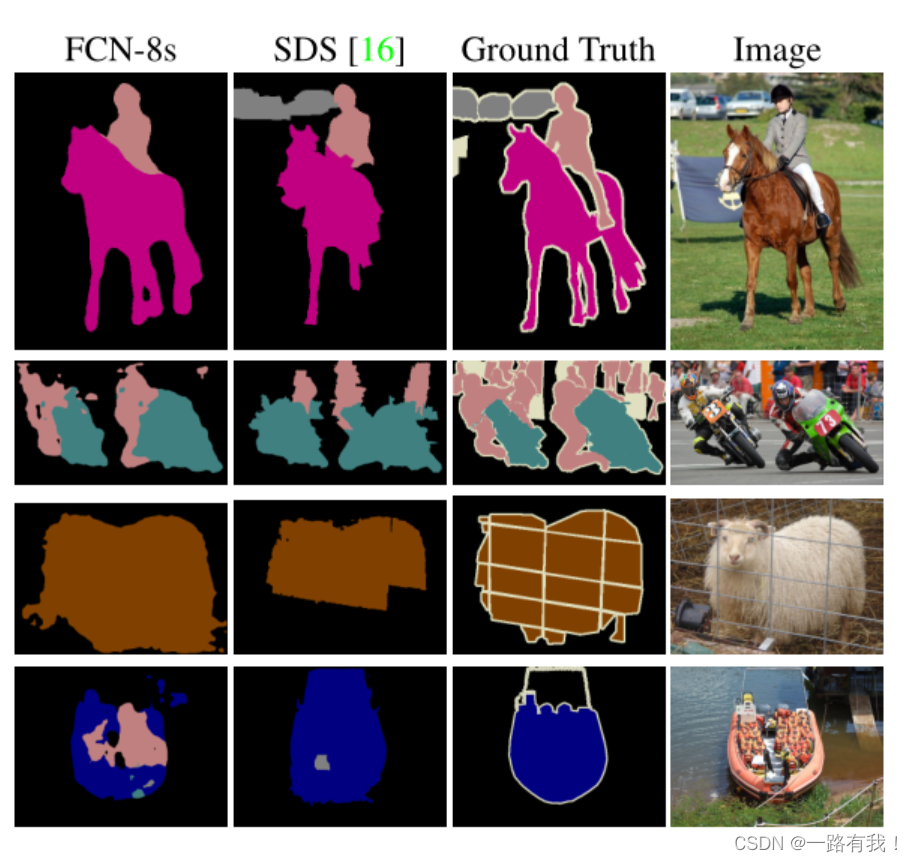
语义分割的目的是对图像中每个像素点进行分类。与普通的分类任务只输出某个类别不同,语义分割任务输出与输入大小相同的图像,输出图像的每个像素对应了输入图像每个像素的类别。语义在图像领域指的是图像的内容,对图片意思的理解,下图是一些语义分割的实例:
模型简介
FCN主要用于图像分割领域,是一种端到端的分割方法,是深度学习应用在图像语义分割的开山之作。通过进行像素级的预测直接得出与原图大小相等的label map。因FCN丢弃全连接层替换为全卷积层,网络所有层均为卷积层,故称为全卷积网络。
全卷积神经网络主要使用以下三种技术:
-
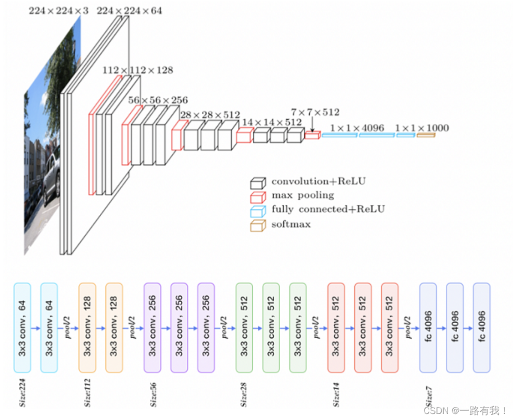
卷积化(Convolutional)
使用VGG-16作为FCN的backbone。VGG-16的输入为224*224的RGB图像,输出为1000个预测值。VGG-16只能接受固定大小的输入,丢弃了空间坐标,产生非空间输出。VGG-16中共有三个全连接层,全连接层也可视为带有覆盖整个区域的卷积。将全连接层转换为卷积层能使网络输出由一维非空间输出变为二维矩阵,利用输出能生成输入图片映射的heatmap。
-
上采样(Upsample)
在卷积过程的卷积操作和池化操作会使得特征图的尺寸变小,为得到原图的大小的稠密图像预测,需要对得到的特征图进行上采样操作。使用双线性插值的参数来初始化上采样逆卷积的参数,后通过反向传播来学习非线性上采样。在网络中执行上采样,以通过像素损失的反向传播进行端到端的学习。
-
跳跃结构(Skip Layer)
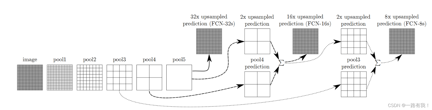
利用上采样技巧对最后一层的特征图进行上采样得到原图大小的分割是步长为32像素的预测,称之为FCN-32s。由于最后一层的特征图太小,损失过多细节,采用skips结构将更具有全局信息的最后一层预测和更浅层的预测结合,使预测结果获取更多的局部细节。将底层(stride 32)的预测(FCN-32s)进行2倍的上采样得到原尺寸的图像,并与从pool4层(stride 16)进行的预测融合起来(相加),这一部分的网络被称为FCN-16s。随后将这一部分的预测再进行一次2倍的上采样并与从pool3层得到的预测融合起来,这一部分的网络被称为FCN-8s。 Skips结构将深层的全局信息与浅层的局部信息相结合。
网络特点
- 不含全连接层(fc)的全卷积(fully conv)网络,可适应任意尺寸输入。
- 增大数据尺寸的反卷积(deconv)层,能够输出精细的结果。
- 结合不同深度层结果的跳级(skip)结构,同时确保鲁棒性和精确性。
数据处理
from download import download

url = "https://mindspore-website.obs.cn-north-4.myhuaweicloud.com/notebook/datasets/dataset_fcn8s.tar"

download(url, "./dataset", kind="tar", replace=True)
数据预处理
由于PASCAL VOC 2012数据集中图像的分辨率大多不一致,无法放在一个tensor中,故输入前需做标准化处理。
数据加载
将PASCAL VOC 2012数据集与SDB数据集进行混合。
import numpy as np
import cv2
import mindspore.dataset as ds

class SegDataset:
    def __init__(self,
                 image_mean,
                 image_std,
                 data_file='',
                 batch_size=32,
                 crop_size=512,
                 max_scale=2.0,
                 min_scale=0.5,
                 ignore_label=255,
                 num_classes=21,
                 num_readers=2,
                 num_parallel_calls=4):

        self.data_file = data_file
        self.batch_size = batch_size
        self.crop_size = crop_size
        self.image_mean = np.array(image_mean, dtype=np.float32)
        self.image_std = np.array(image_std, dtype=np.float32)
        self.max_scale = max_scale
        self.min_scale = min_scale
        self.ignore_label = ignore_label
        self.num_classes = num_classes
        self.num_readers = num_readers
        self.num_parallel_calls = num_parallel_calls
        max_scale > min_scale

    def preprocess_dataset(self, image, label):
        image_out = cv2.imdecode(np.frombuffer(image, dtype=np.uint8), cv2.IMREAD_COLOR)
        label_out = cv2.imdecode(np.frombuffer(label, dtype=np.uint8), cv2.IMREAD_GRAYSCALE)
        sc = np.random.uniform(self.min_scale, self.max_scale)
        new_h, new_w = int(sc * image_out.shape[0]), int(sc * image_out.shape[1])
        image_out = cv2.resize(image_out, (new_w, new_h), interpolation=cv2.INTER_CUBIC)
        label_out = cv2.resize(label_out, (new_w, new_h), interpolation=cv2.INTER_NEAREST)

        image_out = (image_out - self.image_mean) / self.image_std
        out_h, out_w = max(new_h, self.crop_size), max(new_w, self.crop_size)
        pad_h, pad_w = out_h - new_h, out_w - new_w
        if pad_h > 0 or pad_w > 0:
            image_out = cv2.copyMakeBorder(image_out, 0, pad_h, 0, pad_w, cv2.BORDER_CONSTANT, value=0)
            label_out = cv2.copyMakeBorder(label_out, 0, pad_h, 0, pad_w, cv2.BORDER_CONSTANT, value=self.ignore_label)
        offset_h = np.random.randint(0, out_h - self.crop_size + 1)
        offset_w = np.random.randint(0, out_w - self.crop_size + 1)
        image_out = image_out[offset_h: offset_h + self.crop_size, offset_w: offset_w + self.crop_size, :]
        label_out = label_out[offset_h: offset_h + self.crop_size, offset_w: offset_w+self.crop_size]
        if np.random.uniform(0.0, 1.0) > 0.5:
            image_out = image_out[:, ::-1, :]
            label_out = label_out[:, ::-1]
        image_out = image_out.transpose((2, 0, 1))
        image_out = image_out.copy()
        label_out = label_out.copy()
        label_out = label_out.astype("int32")
        return image_out, label_out

    def get_dataset(self):
        ds.config.set_numa_enable(True)
        dataset = ds.MindDataset(self.data_file, columns_list=["data", "label"],
                                 shuffle=True, num_parallel_workers=self.num_readers)
        transforms_list = self.preprocess_dataset
        dataset = dataset.map(operations=transforms_list, input_columns=["data", "label"],
                              output_columns=["data", "label"],
                              num_parallel_workers=self.num_parallel_calls)
        dataset = dataset.shuffle(buffer_size=self.batch_size * 10)
        dataset = dataset.batch(self.batch_size, drop_remainder=True)
        return dataset


# 定义创建数据集的参数
IMAGE_MEAN = [103.53, 116.28, 123.675]
IMAGE_STD = [57.375, 57.120, 58.395]
DATA_FILE = "dataset/dataset_fcn8s/mindname.mindrecord"

# 定义模型训练参数
train_batch_size = 4
crop_size = 512
min_scale = 0.5
max_scale = 2.0
ignore_label = 255
num_classes = 21

# 实例化Dataset
dataset = SegDataset(image_mean=IMAGE_MEAN,
                     image_std=IMAGE_STD,
                     data_file=DATA_FILE,
                     batch_size=train_batch_size,
                     crop_size=crop_size,
                     max_scale=max_scale,
                     min_scale=min_scale,
                     ignore_label=ignore_label,
                     num_classes=num_classes,
                     num_readers=2,
                     num_parallel_calls=4)

dataset = dataset.get_dataset()
训练集可视化
运行以下代码观察载入的数据集图片(数据处理过程中已做归一化处理)。
import numpy as np
import matplotlib.pyplot as plt

plt.figure(figsize=(16, 8))

# 对训练集中的数据进行展示
for i in range(1, 9):
    plt.subplot(2, 4, i)
    show_data = next(dataset.create_dict_iterator())
    show_images = show_data["data"].asnumpy()
    show_images = np.clip(show_images, 0, 1)
# 将图片转换HWC格式后进行展示
    plt.imshow(show_images[0].transpose(1, 2, 0))
    plt.axis("off")
    plt.subplots_adjust(wspace=0.05, hspace=0)
plt.show()
网络构建
网络流程
FCN网络的流程如下图所示:
- 输入图像image,经过pool1池化后,尺寸变为原始尺寸的1/2。
- 经过pool2池化,尺寸变为原始尺寸的1/4。
- 接着经过pool3、pool4、pool5池化,大小分别变为原始尺寸的1/8、1/16、1/32。
- 经过conv6-7卷积,输出的尺寸依然是原图的1/32。
- FCN-32s是最后使用反卷积,使得输出图像大小与输入图像相同。
- FCN-16s是将conv7的输出进行反卷积,使其尺寸扩大两倍至原图的1/16,并将其与pool4输出的特征图进行融合,后通过反卷积扩大到原始尺寸。
- FCN-8s是将conv7的输出进行反卷积扩大4倍,将pool4输出的特征图反卷积扩大2倍,并将pool3输出特征图拿出,三者融合后通反卷积扩大到原始尺寸。
import mindspore.nn as nn

class FCN8s(nn.Cell):
    def __init__(self, n_class):
        super().__init__()
        self.n_class = n_class
        self.conv1 = nn.SequentialCell(
            nn.Conv2d(in_channels=3, out_channels=64,
                      kernel_size=3, weight_init='xavier_uniform'),
            nn.BatchNorm2d(64),
            nn.ReLU(),
            nn.Conv2d(in_channels=64, out_channels=64,
                      kernel_size=3, weight_init='xavier_uniform'),
            nn.BatchNorm2d(64),
            nn.ReLU()
        )
        self.pool1 = nn.MaxPool2d(kernel_size=2, stride=2)
        self.conv2 = nn.SequentialCell(
            nn.Conv2d(in_channels=64, out_channels=128,
                      kernel_size=3, weight_init='xavier_uniform'),
            nn.BatchNorm2d(128),
            nn.ReLU(),
            nn.Conv2d(in_channels=128, out_channels=128,
                      kernel_size=3, weight_init='xavier_uniform'),
            nn.BatchNorm2d(128),
            nn.ReLU()
        )
        self.pool2 = nn.MaxPool2d(kernel_size=2, stride=2)
        self.conv3 = nn.SequentialCell(
            nn.Conv2d(in_channels=128, out_channels=256,
                      kernel_size=3, weight_init='xavier_uniform'),
            nn.BatchNorm2d(256),
            nn.ReLU(),
            nn.Conv2d(in_channels=256, out_channels=256,
                      kernel_size=3, weight_init='xavier_uniform'),
            nn.BatchNorm2d(256),
            nn.ReLU(),
            nn.Conv2d(in_channels=256, out_channels=256,
                      kernel_size=3, weight_init='xavier_uniform'),
            nn.BatchNorm2d(256),
            nn.ReLU()
        )
        self.pool3 = nn.MaxPool2d(kernel_size=2, stride=2)
        self.conv4 = nn.SequentialCell(
            nn.Conv2d(in_channels=256, out_channels=512,
                      kernel_size=3, weight_init='xavier_uniform'),
            nn.BatchNorm2d(512),
            nn.ReLU(),
            nn.Conv2d(in_channels=512, out_channels=512,
                      kernel_size=3, weight_init='xavier_uniform'),
            nn.BatchNorm2d(512),
            nn.ReLU(),
            nn.Conv2d(in_channels=512, out_channels=512,
                      kernel_size=3, weight_init='xavier_uniform'),
            nn.BatchNorm2d(512),
            nn.ReLU()
        )
        self.pool4 = nn.MaxPool2d(kernel_size=2, stride=2)
        self.conv5 = nn.SequentialCell(
            nn.Conv2d(in_channels=512, out_channels=512,
                      kernel_size=3, weight_init='xavier_uniform'),
            nn.BatchNorm2d(512),
            nn.ReLU(),
            nn.Conv2d(in_channels=512, out_channels=512,
                      kernel_size=3, weight_init='xavier_uniform'),
            nn.BatchNorm2d(512),
            nn.ReLU(),
            nn.Conv2d(in_channels=512, out_channels=512,
                      kernel_size=3, weight_init='xavier_uniform'),
            nn.BatchNorm2d(512),
            nn.ReLU()
        )
        self.pool5 = nn.MaxPool2d(kernel_size=2, stride=2)
        self.conv6 = nn.SequentialCell(
            nn.Conv2d(in_channels=512, out_channels=4096,
                      kernel_size=7, weight_init='xavier_uniform'),
            nn.BatchNorm2d(4096),
            nn.ReLU(),
        )
        self.conv7 = nn.SequentialCell(
            nn.Conv2d(in_channels=4096, out_channels=4096,
                      kernel_size=1, weight_init='xavier_uniform'),
            nn.BatchNorm2d(4096),
            nn.ReLU(),
        )
        self.score_fr = nn.Conv2d(in_channels=4096, out_channels=self.n_class,
                                  kernel_size=1, weight_init='xavier_uniform')
        self.upscore2 = nn.Conv2dTranspose(in_channels=self.n_class, out_channels=self.n_class,
                                           kernel_size=4, stride=2, weight_init='xavier_uniform')
        self.score_pool4 = nn.Conv2d(in_channels=512, out_channels=self.n_class,
                                     kernel_size=1, weight_init='xavier_uniform')
        self.upscore_pool4 = nn.Conv2dTranspose(in_channels=self.n_class, out_channels=self.n_class,
                                                kernel_size=4, stride=2, weight_init='xavier_uniform')
        self.score_pool3 = nn.Conv2d(in_channels=256, out_channels=self.n_class,
                                     kernel_size=1, weight_init='xavier_uniform')
        self.upscore8 = nn.Conv2dTranspose(in_channels=self.n_class, out_channels=self.n_class,
                                           kernel_size=16, stride=8, weight_init='xavier_uniform')

    def construct(self, x):
        x1 = self.conv1(x)
        p1 = self.pool1(x1)
        x2 = self.conv2(p1)
        p2 = self.pool2(x2)
        x3 = self.conv3(p2)
        p3 = self.pool3(x3)
        x4 = self.conv4(p3)
        p4 = self.pool4(x4)
        x5 = self.conv5(p4)
        p5 = self.pool5(x5)
        x6 = self.conv6(p5)
        x7 = self.conv7(x6)
        sf = self.score_fr(x7)
        u2 = self.upscore2(sf)
        s4 = self.score_pool4(p4)
        f4 = s4 + u2
        u4 = self.upscore_pool4(f4)
        s3 = self.score_pool3(p3)
        f3 = s3 + u4
        out = self.upscore8(f3)
        return out
训练准备
导入VGG-16部分预训练权重
FCN使用VGG-16作为骨干网络,用于实现图像编码。使用下面代码导入VGG-16预训练模型的部分预训练权重。
from download import download
from mindspore import load_checkpoint, load_param_into_net

url = "https://mindspore-website.obs.cn-north-4.myhuaweicloud.com/notebook/datasets/fcn8s_vgg16_pretrain.ckpt"
download(url, "fcn8s_vgg16_pretrain.ckpt", replace=True)
def load_vgg16():
    ckpt_vgg16 = "fcn8s_vgg16_pretrain.ckpt"
    param_vgg = load_checkpoint(ckpt_vgg16)
    load_param_into_net(net, param_vgg)
损失函数
语义分割是对图像中每个像素点进行分类,仍是分类问题,故损失函数选择交叉熵损失函数来计算FCN网络输出与mask之间的交叉熵损失。这里我们使用的是mindspore.nn.CrossEntropyLoss()作为损失函数。
自定义评价指标 Metrics
这一部分主要对训练出来的模型效果进行评估,为了便于解释,假设如下:共有 𝑘+1 个类(从 𝐿0 到 𝐿𝑘, 其中包含一个空类或背景), 𝑝𝑖𝑗 表示本属于𝑖𝑖类但被预测为𝑗𝑗类的像素数量。即, 𝑝𝑖𝑖𝑝𝑖𝑖 表示真正的数量, 而 𝑝𝑖𝑗,𝑝𝑗𝑖 则分别被解释为假正和假负, 尽管两者都是假正与假负之和。
import numpy as np
import mindspore as ms
import mindspore.nn as nn
import mindspore.train as train

class PixelAccuracy(train.Metric):
    def __init__(self, num_class=21):
        super(PixelAccuracy, self).__init__()
        self.num_class = num_class

    def _generate_matrix(self, gt_image, pre_image):
        mask = (gt_image >= 0) & (gt_image < self.num_class)
        label = self.num_class * gt_image[mask].astype('int') + pre_image[mask]
        count = np.bincount(label, minlength=self.num_class**2)
        confusion_matrix = count.reshape(self.num_class, self.num_class)
        return confusion_matrix

    def clear(self):
        self.confusion_matrix = np.zeros((self.num_class,) * 2)

    def update(self, *inputs):
        y_pred = inputs[0].asnumpy().argmax(axis=1)
        y = inputs[1].asnumpy().reshape(4, 512, 512)
        self.confusion_matrix += self._generate_matrix(y, y_pred)

    def eval(self):
        pixel_accuracy = np.diag(self.confusion_matrix).sum() / self.confusion_matrix.sum()
        return pixel_accuracy


class PixelAccuracyClass(train.Metric):
    def __init__(self, num_class=21):
        super(PixelAccuracyClass, self).__init__()
        self.num_class = num_class

    def _generate_matrix(self, gt_image, pre_image):
        mask = (gt_image >= 0) & (gt_image < self.num_class)
        label = self.num_class * gt_image[mask].astype('int') + pre_image[mask]
        count = np.bincount(label, minlength=self.num_class**2)
        confusion_matrix = count.reshape(self.num_class, self.num_class)
        return confusion_matrix

    def update(self, *inputs):
        y_pred = inputs[0].asnumpy().argmax(axis=1)
        y = inputs[1].asnumpy().reshape(4, 512, 512)
        self.confusion_matrix += self._generate_matrix(y, y_pred)

    def clear(self):
        self.confusion_matrix = np.zeros((self.num_class,) * 2)

    def eval(self):
        mean_pixel_accuracy = np.diag(self.confusion_matrix) / self.confusion_matrix.sum(axis=1)
        mean_pixel_accuracy = np.nanmean(mean_pixel_accuracy)
        return mean_pixel_accuracy


class MeanIntersectionOverUnion(train.Metric):
    def __init__(self, num_class=21):
        super(MeanIntersectionOverUnion, self).__init__()
        self.num_class = num_class

    def _generate_matrix(self, gt_image, pre_image):
        mask = (gt_image >= 0) & (gt_image < self.num_class)
        label = self.num_class * gt_image[mask].astype('int') + pre_image[mask]
        count = np.bincount(label, minlength=self.num_class**2)
        confusion_matrix = count.reshape(self.num_class, self.num_class)
        return confusion_matrix

    def update(self, *inputs):
        y_pred = inputs[0].asnumpy().argmax(axis=1)
        y = inputs[1].asnumpy().reshape(4, 512, 512)
        self.confusion_matrix += self._generate_matrix(y, y_pred)

    def clear(self):
        self.confusion_matrix = np.zeros((self.num_class,) * 2)

    def eval(self):
        mean_iou = np.diag(self.confusion_matrix) / (
            np.sum(self.confusion_matrix, axis=1) + np.sum(self.confusion_matrix, axis=0) -
            np.diag(self.confusion_matrix))
        mean_iou = np.nanmean(mean_iou)
        return mean_iou


class FrequencyWeightedIntersectionOverUnion(train.Metric):
    def __init__(self, num_class=21):
        super(FrequencyWeightedIntersectionOverUnion, self).__init__()
        self.num_class = num_class

    def _generate_matrix(self, gt_image, pre_image):
        mask = (gt_image >= 0) & (gt_image < self.num_class)
        label = self.num_class * gt_image[mask].astype('int') + pre_image[mask]
        count = np.bincount(label, minlength=self.num_class**2)
        confusion_matrix = count.reshape(self.num_class, self.num_class)
        return confusion_matrix

    def update(self, *inputs):
        y_pred = inputs[0].asnumpy().argmax(axis=1)
        y = inputs[1].asnumpy().reshape(4, 512, 512)
        self.confusion_matrix += self._generate_matrix(y, y_pred)

    def clear(self):
        self.confusion_matrix = np.zeros((self.num_class,) * 2)

    def eval(self):
        freq = np.sum(self.confusion_matrix, axis=1) / np.sum(self.confusion_matrix)
        iu = np.diag(self.confusion_matrix) / (
            np.sum(self.confusion_matrix, axis=1) + np.sum(self.confusion_matrix, axis=0) -
            np.diag(self.confusion_matrix))

        frequency_weighted_iou = (freq[freq > 0] * iu[freq > 0]).sum()
        return frequency_weighted_iou
模型训练
导入VGG-16预训练参数后,实例化损失函数、优化器,使用Model接口编译网络,训练FCN-8s网络。
import mindspore
from mindspore import Tensor
import mindspore.nn as nn
from mindspore.train import ModelCheckpoint, CheckpointConfig, LossMonitor, TimeMonitor, Model

device_target = "Ascend"
mindspore.set_context(mode=mindspore.PYNATIVE_MODE, device_target=device_target)

train_batch_size = 4
num_classes = 21
# 初始化模型结构
net = FCN8s(n_class=21)
# 导入vgg16预训练参数
load_vgg16()
# 计算学习率
min_lr = 0.0005
base_lr = 0.05
train_epochs = 1
iters_per_epoch = dataset.get_dataset_size()
total_step = iters_per_epoch * train_epochs

lr_scheduler = mindspore.nn.cosine_decay_lr(min_lr,
                                            base_lr,
                                            total_step,
                                            iters_per_epoch,
                                            decay_epoch=2)
lr = Tensor(lr_scheduler[-1])

# 定义损失函数
loss = nn.CrossEntropyLoss(ignore_index=255)
# 定义优化器
optimizer = nn.Momentum(params=net.trainable_params(), learning_rate=lr, momentum=0.9, weight_decay=0.0001)
# 定义loss_scale
scale_factor = 4
scale_window = 3000
loss_scale_manager = ms.amp.DynamicLossScaleManager(scale_factor, scale_window)
# 初始化模型
if device_target == "Ascend":
    model = Model(net, loss_fn=loss, optimizer=optimizer, loss_scale_manager=loss_scale_manager, metrics={"pixel accuracy": PixelAccuracy(), "mean pixel accuracy": PixelAccuracyClass(), "mean IoU": MeanIntersectionOverUnion(), "frequency weighted IoU": FrequencyWeightedIntersectionOverUnion()})
else:
    model = Model(net, loss_fn=loss, optimizer=optimizer, metrics={"pixel accuracy": PixelAccuracy(), "mean pixel accuracy": PixelAccuracyClass(), "mean IoU": MeanIntersectionOverUnion(), "frequency weighted IoU": FrequencyWeightedIntersectionOverUnion()})

# 设置ckpt文件保存的参数
time_callback = TimeMonitor(data_size=iters_per_epoch)
loss_callback = LossMonitor()
callbacks = [time_callback, loss_callback]
save_steps = 330
keep_checkpoint_max = 5
config_ckpt = CheckpointConfig(save_checkpoint_steps=10,
                               keep_checkpoint_max=keep_checkpoint_max)
ckpt_callback = ModelCheckpoint(prefix="FCN8s",
                                directory="./ckpt",
                                config=config_ckpt)
callbacks.append(ckpt_callback)
model.train(train_epochs, dataset, callbacks=callbacks)
因为FCN网络在训练的过程中需要大量的训练数据和训练轮数,这里只提供了小数据单个epoch的训练来演示loss收敛的过程,下文中使用已训练好的权重文件进行模型评估和推理效果的展示。
模型评估
IMAGE_MEAN = [103.53, 116.28, 123.675]
IMAGE_STD = [57.375, 57.120, 58.395]
DATA_FILE = "dataset/dataset_fcn8s/mindname.mindrecord"

# 下载已训练好的权重文件
url = "https://mindspore-website.obs.cn-north-4.myhuaweicloud.com/notebook/datasets/FCN8s.ckpt"
download(url, "FCN8s.ckpt", replace=True)
net = FCN8s(n_class=num_classes)

ckpt_file = "FCN8s.ckpt"
param_dict = load_checkpoint(ckpt_file)
load_param_into_net(net, param_dict)

if device_target == "Ascend":
    model = Model(net, loss_fn=loss, optimizer=optimizer, loss_scale_manager=loss_scale_manager, metrics={"pixel accuracy": PixelAccuracy(), "mean pixel accuracy": PixelAccuracyClass(), "mean IoU": MeanIntersectionOverUnion(), "frequency weighted IoU": FrequencyWeightedIntersectionOverUnion()})
else:
    model = Model(net, loss_fn=loss, optimizer=optimizer, metrics={"pixel accuracy": PixelAccuracy(), "mean pixel accuracy": PixelAccuracyClass(), "mean IoU": MeanIntersectionOverUnion(), "frequency weighted IoU": FrequencyWeightedIntersectionOverUnion()})

# 实例化Dataset
dataset = SegDataset(image_mean=IMAGE_MEAN,
                     image_std=IMAGE_STD,
                     data_file=DATA_FILE,
                     batch_size=train_batch_size,
                     crop_size=crop_size,
                     max_scale=max_scale,
                     min_scale=min_scale,
                     ignore_label=ignore_label,
                     num_classes=num_classes,
                     num_readers=2,
                     num_parallel_calls=4)
dataset_eval = dataset.get_dataset()
model.eval(dataset_eval)
模型推理
使用训练的网络对模型推理结果进行展示。
import cv2
import matplotlib.pyplot as plt

net = FCN8s(n_class=num_classes)
# 设置超参
ckpt_file = "FCN8s.ckpt"
param_dict = load_checkpoint(ckpt_file)
load_param_into_net(net, param_dict)
eval_batch_size = 4
img_lst = []
mask_lst = []
res_lst = []
# 推理效果展示(上方为输入图片,下方为推理效果图片)
plt.figure(figsize=(8, 5))
show_data = next(dataset_eval.create_dict_iterator())
show_images = show_data["data"].asnumpy()
mask_images = show_data["label"].reshape([4, 512, 512])
show_images = np.clip(show_images, 0, 1)
for i in range(eval_batch_size):
    img_lst.append(show_images[i])
    mask_lst.append(mask_images[i])
res = net(show_data["data"]).asnumpy().argmax(axis=1)
for i in range(eval_batch_size):
    plt.subplot(2, 4, i + 1)
    plt.imshow(img_lst[i].transpose(1, 2, 0))
    plt.axis("off")
    plt.subplots_adjust(wspace=0.05, hspace=0.02)
    plt.subplot(2, 4, i + 5)
    plt.imshow(res[i])
    plt.axis("off")
    plt.subplots_adjust(wspace=0.05, hspace=0.02)
plt.show()
总结
FCN的核心贡献在于提出使用全卷积层,通过学习让图片实现端到端分割。与传统使用CNN进行图像分割的方法相比,FCN有两大明显的优点:一是可以接受任意大小的输入图像,无需要求所有的训练图像和测试图像具有固定的尺寸。二是更加高效,避免了由于使用像素块而带来的重复存储和计算卷积的问题。
同时FCN网络也存在待改进之处:
一是得到的结果仍不够精细。进行8倍上采样虽然比32倍的效果好了很多,但是上采样的结果仍比较模糊和平滑,尤其是边界处,网络对图像中的细节不敏感。 二是对各个像素进行分类,没有充分考虑像素与像素之间的关系(如不连续性和相似性)。忽略了在通常的基于像素分类的分割方法中使用的空间规整(spatial regularization)步骤,缺乏空间一致性。
引用
[1]Long, Jonathan, Evan Shelhamer, and Trevor Darrell. "Fully convolutional networks for Semantic Segmentation." Proceedings of the IEEE Conference on Computer Vision and Pattern Recognition. 2015.
ResNet50迁移学习
在实际应用场景中,由于训练数据集不足,所以很少有人会从头开始训练整个网络。普遍的做法是,在一个非常大的基础数据集上训练得到一个预训练模型,然后使用该模型来初始化网络的权重参数或作为固定特征提取器应用于特定的任务中。本章将使用迁移学习的方法对ImageNet数据集中的狼和狗图像进行分类。
数据准备
下载数据集
下载案例所用到的狗与狼分类数据集,数据集中的图像来自于ImageNet,每个分类有大约120张训练图像与30张验证图像。使用download接口下载数据集,并将下载后的数据集自动解压到当前目录下。
from download import download

dataset_url = "https://mindspore-website.obs.cn-north-4.myhuaweicloud.com/notebook/datasets/intermediate/Canidae_data.zip"

download(dataset_url, "./datasets-Canidae", kind="zip", replace=True)
加载数据集
狼狗数据集提取自ImageNet分类数据集,使用mindspore.dataset.ImageFolderDataset接口来加载数据集,并进行相关图像增强操作。
首先执行过程定义一些输入:
batch_size = 18                             # 批量大小
image_size = 224                            # 训练图像空间大小
num_epochs = 5                             # 训练周期数
lr = 0.001                                  # 学习率
momentum = 0.9                              # 动量
workers = 4

import mindspore as ms
import mindspore.dataset as ds
import mindspore.dataset.vision as vision

# 数据集目录路径
data_path_train = "./datasets-Canidae/data/Canidae/train/"
data_path_val = "./datasets-Canidae/data/Canidae/val/"

# 创建训练数据集

def create_dataset_canidae(dataset_path, usage):
    """数据加载"""
    data_set = ds.ImageFolderDataset(dataset_path,
                                     num_parallel_workers=workers,
                                     shuffle=True,)

    # 数据增强操作
    mean = [0.485 * 255, 0.456 * 255, 0.406 * 255]
    std = [0.229 * 255, 0.224 * 255, 0.225 * 255]
    scale = 32

    if usage == "train":
        # Define map operations for training dataset
        trans = [
            vision.RandomCropDecodeResize(size=image_size, scale=(0.08, 1.0), ratio=(0.75, 1.333)),
            vision.RandomHorizontalFlip(prob=0.5),
            vision.Normalize(mean=mean, std=std),
            vision.HWC2CHW()
        ]
    else:
        # Define map operations for inference dataset
        trans = [
            vision.Decode(),
            vision.Resize(image_size + scale),
            vision.CenterCrop(image_size),
            vision.Normalize(mean=mean, std=std),
            vision.HWC2CHW()
        ]


    # 数据映射操作
    data_set = data_set.map(
        operations=trans,
        input_columns='image',
        num_parallel_workers=workers)


    # 批量操作
    data_set = data_set.batch(batch_size)

    return data_set


dataset_train = create_dataset_canidae(data_path_train, "train")
step_size_train = dataset_train.get_dataset_size()

dataset_val = create_dataset_canidae(data_path_val, "val")
step_size_val = dataset_val.get_dataset_size()
数据集可视化
从mindspore.dataset.ImageFolderDataset接口中加载的训练数据集返回值为字典,用户可通过 create_dict_iterator 接口创建数据迭代器,使用 next 迭代访问数据集。本章中 batch_size 设为18,所以使用 next 一次可获取18个图像及标签数据。
data = next(dataset_train.create_dict_iterator())
images = data["image"]
labels = data["label"]

print("Tensor of image", images.shape)
print("Labels:", labels)
对获取到的图像及标签数据进行可视化,标题为图像对应的label名称。
import matplotlib.pyplot as plt
import numpy as np

# class_name对应label,按文件夹字符串从小到大的顺序标记label
class_name = {0: "dogs", 1: "wolves"}

plt.figure(figsize=(5, 5))
for i in range(4):
    # 获取图像及其对应的label
    data_image = images[i].asnumpy()
    data_label = labels[i]
    # 处理图像供展示使用
    data_image = np.transpose(data_image, (1, 2, 0))
    mean = np.array([0.485, 0.456, 0.406])
    std = np.array([0.229, 0.224, 0.225])
    data_image = std * data_image + mean
    data_image = np.clip(data_image, 0, 1)
    # 显示图像
    plt.subplot(2, 2, i+1)
    plt.imshow(data_image)
    plt.title(class_name[int(labels[i].asnumpy())])
    plt.axis("off")

plt.show()
训练模型
本章使用ResNet50模型进行训练。搭建好模型框架后,通过将pretrained参数设置为True来下载ResNet50的预训练模型并将权重参数加载到网络中。
构建Resnet50网络
from typing import Type, Union, List, Optional
from mindspore import nn, train
from mindspore.common.initializer import Normal


weight_init = Normal(mean=0, sigma=0.02)
gamma_init = Normal(mean=1, sigma=0.02)

class ResidualBlockBase(nn.Cell):
    expansion: int = 1  # 最后一个卷积核数量与第一个卷积核数量相等

    def __init__(self, in_channel: int, out_channel: int,
                 stride: int = 1, norm: Optional[nn.Cell] = None,
                 down_sample: Optional[nn.Cell] = None) -> None:
        super(ResidualBlockBase, self).__init__()
        if not norm:
            self.norm = nn.BatchNorm2d(out_channel)
        else:
            self.norm = norm

        self.conv1 = nn.Conv2d(in_channel, out_channel,
                               kernel_size=3, stride=stride,
                               weight_init=weight_init)
        self.conv2 = nn.Conv2d(in_channel, out_channel,
                               kernel_size=3, weight_init=weight_init)
        self.relu = nn.ReLU()
        self.down_sample = down_sample

    def construct(self, x):
        """ResidualBlockBase construct."""
        identity = x  # shortcuts分支

        out = self.conv1(x)  # 主分支第一层:3*3卷积层
        out = self.norm(out)
        out = self.relu(out)
        out = self.conv2(out)  # 主分支第二层:3*3卷积层
        out = self.norm(out)

        if self.down_sample is not None:
            identity = self.down_sample(x)
        out += identity  # 输出为主分支与shortcuts之和
        out = self.relu(out)

        return out

class ResidualBlock(nn.Cell):
    expansion = 4  # 最后一个卷积核的数量是第一个卷积核数量的4倍

    def __init__(self, in_channel: int, out_channel: int,
                 stride: int = 1, down_sample: Optional[nn.Cell] = None) -> None:
        super(ResidualBlock, self).__init__()

        self.conv1 = nn.Conv2d(in_channel, out_channel,
                               kernel_size=1, weight_init=weight_init)
        self.norm1 = nn.BatchNorm2d(out_channel)
        self.conv2 = nn.Conv2d(out_channel, out_channel,
                               kernel_size=3, stride=stride,
                               weight_init=weight_init)
        self.norm2 = nn.BatchNorm2d(out_channel)
        self.conv3 = nn.Conv2d(out_channel, out_channel * self.expansion,
                               kernel_size=1, weight_init=weight_init)
        self.norm3 = nn.BatchNorm2d(out_channel * self.expansion)

        self.relu = nn.ReLU()
        self.down_sample = down_sample

    def construct(self, x):

        identity = x  # shortscuts分支

        out = self.conv1(x)  # 主分支第一层:1*1卷积层
        out = self.norm1(out)
        out = self.relu(out)
        out = self.conv2(out)  # 主分支第二层:3*3卷积层
        out = self.norm2(out)
        out = self.relu(out)
        out = self.conv3(out)  # 主分支第三层:1*1卷积层
        out = self.norm3(out)

        if self.down_sample is not None:
            identity = self.down_sample(x)

        out += identity  # 输出为主分支与shortcuts之和
        out = self.relu(out)

        return out

def make_layer(last_out_channel, block: Type[Union[ResidualBlockBase, ResidualBlock]],
               channel: int, block_nums: int, stride: int = 1):
    down_sample = None  # shortcuts分支


    if stride != 1 or last_out_channel != channel * block.expansion:

        down_sample = nn.SequentialCell([
            nn.Conv2d(last_out_channel, channel * block.expansion,
                      kernel_size=1, stride=stride, weight_init=weight_init),
            nn.BatchNorm2d(channel * block.expansion, gamma_init=gamma_init)
        ])

    layers = []
    layers.append(block(last_out_channel, channel, stride=stride, down_sample=down_sample))

    in_channel = channel * block.expansion
    # 堆叠残差网络
    for _ in range(1, block_nums):

        layers.append(block(in_channel, channel))

    return nn.SequentialCell(layers)

from mindspore import load_checkpoint, load_param_into_net


class ResNet(nn.Cell):
    def __init__(self, block: Type[Union[ResidualBlockBase, ResidualBlock]],
                 layer_nums: List[int], num_classes: int, input_channel: int) -> None:
        super(ResNet, self).__init__()

        self.relu = nn.ReLU()
        # 第一个卷积层,输入channel为3(彩色图像),输出channel为64
        self.conv1 = nn.Conv2d(3, 64, kernel_size=7, stride=2, weight_init=weight_init)
        self.norm = nn.BatchNorm2d(64)
        # 最大池化层,缩小图片的尺寸
        self.max_pool = nn.MaxPool2d(kernel_size=3, stride=2, pad_mode='same')
        # 各个残差网络结构块定义,
        self.layer1 = make_layer(64, block, 64, layer_nums[0])
        self.layer2 = make_layer(64 * block.expansion, block, 128, layer_nums[1], stride=2)
        self.layer3 = make_layer(128 * block.expansion, block, 256, layer_nums[2], stride=2)
        self.layer4 = make_layer(256 * block.expansion, block, 512, layer_nums[3], stride=2)
        # 平均池化层
        self.avg_pool = nn.AvgPool2d()
        # flattern层
        self.flatten = nn.Flatten()
        # 全连接层
        self.fc = nn.Dense(in_channels=input_channel, out_channels=num_classes)

    def construct(self, x):

        x = self.conv1(x)
        x = self.norm(x)
        x = self.relu(x)
        x = self.max_pool(x)

        x = self.layer1(x)
        x = self.layer2(x)
        x = self.layer3(x)
        x = self.layer4(x)

        x = self.avg_pool(x)
        x = self.flatten(x)
        x = self.fc(x)

        return x


def _resnet(model_url: str, block: Type[Union[ResidualBlockBase, ResidualBlock]],
            layers: List[int], num_classes: int, pretrained: bool, pretrianed_ckpt: str,
            input_channel: int):
    model = ResNet(block, layers, num_classes, input_channel)

    if pretrained:
        # 加载预训练模型
        download(url=model_url, path=pretrianed_ckpt, replace=True)
        param_dict = load_checkpoint(pretrianed_ckpt)
        load_param_into_net(model, param_dict)

    return model


def resnet50(num_classes: int = 1000, pretrained: bool = False):
    "ResNet50模型"
    resnet50_url = "https://mindspore-website.obs.cn-north-4.myhuaweicloud.com/notebook/models/application/resnet50_224_new.ckpt"
    resnet50_ckpt = "./LoadPretrainedModel/resnet50_224_new.ckpt"
    return _resnet(resnet50_url, ResidualBlock, [3, 4, 6, 3], num_classes,
                   pretrained, resnet50_ckpt, 2048)
固定特征进行训练
使用固定特征进行训练的时候,需要冻结除最后一层之外的所有网络层。通过设置 requires_grad == False 冻结参数,以便不在反向传播中计算梯度。
import mindspore as ms
import matplotlib.pyplot as plt
import os
import time

net_work = resnet50(pretrained=True)

# 全连接层输入层的大小
in_channels = net_work.fc.in_channels
# 输出通道数大小为狼狗分类数2
head = nn.Dense(in_channels, 2)
# 重置全连接层
net_work.fc = head

# 平均池化层kernel size为7
avg_pool = nn.AvgPool2d(kernel_size=7)
# 重置平均池化层
net_work.avg_pool = avg_pool

# 冻结除最后一层外的所有参数
for param in net_work.get_parameters():
    if param.name not in ["fc.weight", "fc.bias"]:
        param.requires_grad = False

# 定义优化器和损失函数
opt = nn.Momentum(params=net_work.trainable_params(), learning_rate=lr, momentum=0.5)
loss_fn = nn.SoftmaxCrossEntropyWithLogits(sparse=True, reduction='mean')


def forward_fn(inputs, targets):
    logits = net_work(inputs)
    loss = loss_fn(logits, targets)

    return loss

grad_fn = ms.value_and_grad(forward_fn, None, opt.parameters)

def train_step(inputs, targets):
    loss, grads = grad_fn(inputs, targets)
    opt(grads)
    return loss

# 实例化模型
model1 = train.Model(net_work, loss_fn, opt, metrics={"Accuracy": train.Accuracy()})
训练和评估
开始训练模型,与没有预训练模型相比,将节约一大半时间,因为此时可以不用计算部分梯度。保存评估精度最高的ckpt文件于当前路径的./BestCheckpoint/resnet50-best-freezing-param.ckpt。
import mindspore as ms
import matplotlib.pyplot as plt
import os
import time
dataset_train = create_dataset_canidae(data_path_train, "train")
step_size_train = dataset_train.get_dataset_size()

dataset_val = create_dataset_canidae(data_path_val, "val")
step_size_val = dataset_val.get_dataset_size()

num_epochs = 5

# 创建迭代器
data_loader_train = dataset_train.create_tuple_iterator(num_epochs=num_epochs)
data_loader_val = dataset_val.create_tuple_iterator(num_epochs=num_epochs)
best_ckpt_dir = "./BestCheckpoint"
best_ckpt_path = "./BestCheckpoint/resnet50-best-freezing-param.ckpt"

import mindspore as ms
import matplotlib.pyplot as plt
import os
import time
# 开始循环训练
print("Start Training Loop ...")

best_acc = 0

for epoch in range(num_epochs):
    losses = []
    net_work.set_train()

    epoch_start = time.time()

    # 为每轮训练读入数据
    for i, (images, labels) in enumerate(data_loader_train):
        labels = labels.astype(ms.int32)
        loss = train_step(images, labels)
        losses.append(loss)

    # 每个epoch结束后,验证准确率

    acc = model1.eval(dataset_val)['Accuracy']

    epoch_end = time.time()
    epoch_seconds = (epoch_end - epoch_start) * 1000
    step_seconds = epoch_seconds/step_size_train

    print("-" * 20)
    print("Epoch: [%3d/%3d], Average Train Loss: [%5.3f], Accuracy: [%5.3f]" % (
        epoch+1, num_epochs, sum(losses)/len(losses), acc
    ))
    print("epoch time: %5.3f ms, per step time: %5.3f ms" % (
        epoch_seconds, step_seconds
    ))

    if acc > best_acc:
        best_acc = acc
        if not os.path.exists(best_ckpt_dir):
            os.mkdir(best_ckpt_dir)
        ms.save_checkpoint(net_work, best_ckpt_path)

print("=" * 80)
print(f"End of validation the best Accuracy is: {best_acc: 5.3f}, "
      f"save the best ckpt file in {best_ckpt_path}", flush=True)
可视化模型预测
使用固定特征得到的best.ckpt文件对对验证集的狼和狗图像数据进行预测。若预测字体为蓝色即为预测正确,若预测字体为红色则预测错误。
import matplotlib.pyplot as plt
import mindspore as ms

def visualize_model(best_ckpt_path, val_ds):
    net = resnet50()
    # 全连接层输入层的大小
    in_channels = net.fc.in_channels
    # 输出通道数大小为狼狗分类数2
    head = nn.Dense(in_channels, 2)
    # 重置全连接层
    net.fc = head
    # 平均池化层kernel size为7
    avg_pool = nn.AvgPool2d(kernel_size=7)
    # 重置平均池化层
    net.avg_pool = avg_pool
    # 加载模型参数
    param_dict = ms.load_checkpoint(best_ckpt_path)
    ms.load_param_into_net(net, param_dict)
    model = train.Model(net)
    # 加载验证集的数据进行验证
    data = next(val_ds.create_dict_iterator())
    images = data["image"].asnumpy()
    labels = data["label"].asnumpy()
    class_name = {0: "dogs", 1: "wolves"}
    # 预测图像类别
    output = model.predict(ms.Tensor(data['image']))
    pred = np.argmax(output.asnumpy(), axis=1)

    # 显示图像及图像的预测值
    plt.figure(figsize=(5, 5))
    for i in range(4):
        plt.subplot(2, 2, i + 1)
        # 若预测正确,显示为蓝色;若预测错误,显示为红色
        color = 'blue' if pred[i] == labels[i] else 'red'
        plt.title('predict:{}'.format(class_name[pred[i]]), color=color)
        picture_show = np.transpose(images[i], (1, 2, 0))
        mean = np.array([0.485, 0.456, 0.406])
        std = np.array([0.229, 0.224, 0.225])
        picture_show = std * picture_show + mean
        picture_show = np.clip(picture_show, 0, 1)
        plt.imshow(picture_show)
        plt.axis('off')

    plt.show()

visualize_model(best_ckpt_path, dataset_val)
最后打卡今天的学习时间
心得
今天我学习了FCN图像语义分割和ResNet50迁移学习。FCN是一种用于图像语义分割的框架,通过进行像素级预测,可以应用于人脸识别、物体检测、医学影像等领域。语义分割的目标是对图像中每个像素点进行分类,生成与输入图像大小相同的输出图像。迁移学习则利用预训练的ResNet50模型来处理图像分类任务,通过在大规模数据集上预训练模型,再将其应用于具体任务,可以有效解决训练数据不足的问题。今天的学习让我掌握了语义分割和迁移学习的基础知识,为图像处理和分类任务奠定了基础。

昇腾计算产业是基于昇腾系列(HUAWEI Ascend)处理器和基础软件构建的全栈 AI计算基础设施、行业应用及服务,https://devpress.csdn.net/organization/setting/general/146749包括昇腾系列处理器、系列硬件、CANN、AI计算框架、应用使能、开发工具链、管理运维工具、行业应用及服务等全产业链
更多推荐

 20
20 0
0- 0


 已为社区贡献16条内容

所有评论(0)