☀️ 最近报名参加了昇思25天学习打卡训练营
☀️ 昨天初步学习了MindSpore的基本操作
☀️ 第二天学习 初学入门 / 初学教程 / 03-张量 Tensor

1. 代码跑通流程

张量（Tensor）是一个可用来表示在一些矢量、标量和其他张量之间的线性关系的多线性函数，这些线性关系的基本例子有内积、外积、线性映射以及笛卡儿积。其坐标在 𝑛 维空间内，有  𝑛^𝑟 个分量的一种量，其中每个分量都是坐标的函数，而在坐标变换时，这些分量也依照某些规则作线性变换。 𝑟 称为该张量的秩或阶（与矩阵的秩和阶均无关系）。

张量是一种特殊的数据结构，与数组和矩阵非常相似。张量（Tensor）是MindSpore网络运算中的基本数据结构，这里主要介绍张量和稀疏张量的属性及用法。

1.1 导入库

import numpy as np
import mindspore
from mindspore import ops
from mindspore import Tensor, CSRTensor, COOTensor

1.2 创建张量

张量的创建方式有多种，构造张量时，支持传入Tensor、float、int、bool、tuple、list和numpy.ndarray类型。

1️⃣ 根据数据直接生成：可以根据数据创建张量，数据类型可以设置或者通过框架自动推断。

data = [1, 0, 1, 0]
x_data = Tensor(data)
print(x_data, x_data.shape, x_data.dtype)

输出：

[1 0 1 0] (4,) Int64

2️⃣ 从NumPy数组生成：可以从NumPy数组创建张量。

np_array = np.array(data)
x_np = Tensor(np_array)
print(x_np, x_np.shape, x_np.dtype)

输出：

[1 0 1 0] (4,) Int64

3️⃣ 使用init初始化器构造张量：当使用init初始化器对张量进行初始化时，支持传入的参数有init、shape、dtype。

• init: 支持传入initializer的子类。如：下方示例中的 One() 和 Normal()。
• shape: 支持传入 list、tuple、 int。
• dtype: 支持传入mindspore.dtype。

from mindspore.common.initializer import One, Normal

# Initialize a tensor with ones
tensor1 = mindspore.Tensor(shape=(2, 2), dtype=mindspore.float32, init=One())
# Initialize a tensor from normal distribution
tensor2 = mindspore.Tensor(shape=(2, 2), dtype=mindspore.float32, init=Normal())

print("tensor1:\n", tensor1)
print("tensor2:\n", tensor2)

Normal()：正态分布随机数的生成函数

输出：

tensor1:
 [[1. 1.]
 [1. 1.]]
tensor2:
 [[ 0.00117931  0.00447294]
 [-0.00659744  0.01019117]]

init主要用于并行模式下的延后初始化，在正常情况下不建议使用init对参数进行初始化。

4️⃣ 继承另一个张量的属性，形成新的张量

from mindspore import ops

x_ones = ops.ones_like(x_data)
print(f"Ones Tensor: \n {x_ones} \n")

x_zeros = ops.zeros_like(x_data)
print(f"Zeros Tensor: \n {x_zeros} \n")

输出：

Ones Tensor: 
 [1 1 1 1] 

Zeros Tensor: 
 [0 0 0 0] 

1.3 张量属性

张量的属性包括形状、数据类型、转置张量、单个元素大小、占用字节数量、维数、元素个数和每一维步长。

• 形状（shape）：Tensor的shape，是一个tuple。
• 数据类型（dtype）：Tensor的dtype，是MindSpore的一个数据类型。
• 单个元素大小（itemsize）： Tensor中每一个元素占用字节数，是一个整数。
• 占用字节数量（nbytes）： Tensor占用的总字节数，是一个整数。
• 维数（ndim）： Tensor的秩，也就是len(tensor.shape)，是一个整数。
• 元素个数（size）： Tensor中所有元素的个数，是一个整数。
• 每一维步长（strides）： Tensor每一维所需要的字节数，是一个tuple。

x = Tensor(np.array([[1, 2], [3, 4]]), mindspore.int32)

print("x_shape:", x.shape)
print("x_dtype:", x.dtype)
print("x_itemsize:", x.itemsize)
print("x_nbytes:", x.nbytes)
print("x_ndim:", x.ndim)
print("x_size:", x.size)
print("x_strides:", x.strides)

输出：

x_shape: (2, 2)
x_dtype: Int32
x_itemsize: 4
x_nbytes: 16
x_ndim: 2
x_size: 4
x_strides: (8, 4)

1.4 张量运算

张量之间有很多运算，包括算术、线性代数、矩阵处理（转置、标引、切片）、采样等，张量运算和NumPy的使用方式类似，下面介绍其中几种操作。

1️⃣ 普通算术运算有：加（+）、减（-）、乘（*）、除（/）、取模（%）、整除（//）。

x = Tensor(np.array([1, 2, 3]), mindspore.float32)
y = Tensor(np.array([4, 5, 6]), mindspore.float32)

output_add = x + y
output_sub = x - y
output_mul = x * y
output_div = y / x
output_mod = y % x
output_floordiv = y // x

print("add:", output_add)
print("sub:", output_sub)
print("mul:", output_mul)
print("div:", output_div)
print("mod:", output_mod)
print("floordiv:", output_floordiv)

输出：

add: [5. 7. 9.]
sub: [-3. -3. -3.]
mul: [ 4. 10. 18.]
div: [4.  2.5 2. ]
mod: [0. 1. 0.]
floordiv: [4. 2. 2.]

这些比较简单，可以用手算验证一下对不对

2️⃣ concat将给定维度上的一系列张量连接起来。

data1 = Tensor(np.array([[0, 1], [2, 3]]).astype(np.float32))
data2 = Tensor(np.array([[4, 5], [6, 7]]).astype(np.float32))
output = ops.concat((data1, data2), axis=0)

print(output)
print("shape:\n", output.shape)

输出：

[[0. 1.]
 [2. 3.]
 [4. 5.]
 [6. 7.]]
shape:
 (4, 2)

3️⃣ stack则是从另一个维度上将两个张量合并起来。

data1 = Tensor(np.array([[0, 1], [2, 3]]).astype(np.float32))
data2 = Tensor(np.array([[4, 5], [6, 7]]).astype(np.float32))
output = ops.stack([data1, data2])

print(output)
print("shape:\n", output.shape)

输出：

[[[0. 1.]
  [2. 3.]]

 [[4. 5.]
  [6. 7.]]]
shape:
 (2, 2, 2)

📝 注意 concat 和 stack 的区别：
concat是对dim进行拼接，stack是对dim维进行堆叠。
concat不会增加新的维度，在指定维度上拼接。
stack增加一个新的维度将两个单位，然后再上一维度分别进行堆叠。

1.5 Tensor与NumPy转换

Tensor可以和NumPy进行互相转换。

1️⃣ Tensor转换为NumPy
与张量创建相同，使用 Tensor.asnumpy() 将Tensor变量转换为NumPy变量。

t = Tensor([1., 1., 1., 1., 1.])
print(f"t: {t}", type(t))
n = t.asnumpy()
print(f"n: {n}", type(n))

输出：

t: [1. 1. 1. 1. 1.] <class 'mindspore.common.tensor.Tensor'>
n: [1. 1. 1. 1. 1.] <class 'numpy.ndarray'>

2️⃣ NumPy转换为Tensor
使用 Tensor.from_numpy() 将NumPy变量转换为Tensor变量。

n = np.ones(5)
t = Tensor.from_numpy(n)
np.add(n, 1, out=n)
print(f"n: {n}", type(n))
print(f"t: {t}", type(t))

输出：

n: [2. 2. 2. 2. 2.] <class 'numpy.ndarray'>
t: [2. 2. 2. 2. 2.] <class 'mindspore.common.tensor.Tensor'>

1.6 稀疏张量

稀疏张量是一种特殊张量，其中绝大部分元素的值为零。

在某些应用场景中（比如推荐系统、分子动力学、图神经网络等），数据的特征是稀疏的，若使用普通张量表征这些数据会引入大量不必要的计算、存储和通讯开销。这时就可以使用稀疏张量来表征这些数据。

MindSpore现在已经支持最常用的CSR和COO两种稀疏数据格式。

常用稀疏张量的表达形式是 <indices:Tensor, values:Tensor, shape:Tensor> 。其中，indices 表示非零下标元素， values 表示非零元素的值，shape 表示的是被压缩的稀疏张量的形状。在这个结构下，我们定义了三种稀疏张量结构：CSRTensor、COOTensor和RowTensor。

1️⃣ CSRTensor
CSR（Compressed Sparse Row）稀疏张量格式有着高效的存储与计算的优势。其中，非零元素的值存储在values中，非零元素的位置存储在indptr（行）和indices（列）中。各参数含义如下：

• indptr: 一维整数张量, 表示稀疏数据每一行的非零元素在values中的起始位置和终止位置, 索引数据类型支持int16、int32、int64。注意：For CSRTensor, indptr must have length (1 + shape[0])
• indices: 一维整数张量，表示稀疏张量非零元素在列中的位置, 与values长度相等，索引数据类型支持int16、int32、int64。
• values: 一维张量，表示CSRTensor相对应的非零元素的值，与indices长度相等。
• shape: 表示被压缩的稀疏张量的形状，数据类型为Tuple，目前仅支持二维CSRTensor。

indptr = Tensor([0, 1, 2])
indices = Tensor([0, 1])
values = Tensor([1, 2], dtype=mindspore.float32)
shape = (2, 4)

# Make a CSRTensor
csr_tensor = CSRTensor(indptr, indices, values, shape)

print(csr_tensor.astype(mindspore.float64).dtype)

输出：

Float64

如果想要看稠密形式的：

print(csr_tensor.to_dense())

输出：

[[1. 0. 0. 0.]
 [0. 2. 0. 0.]]

再比如：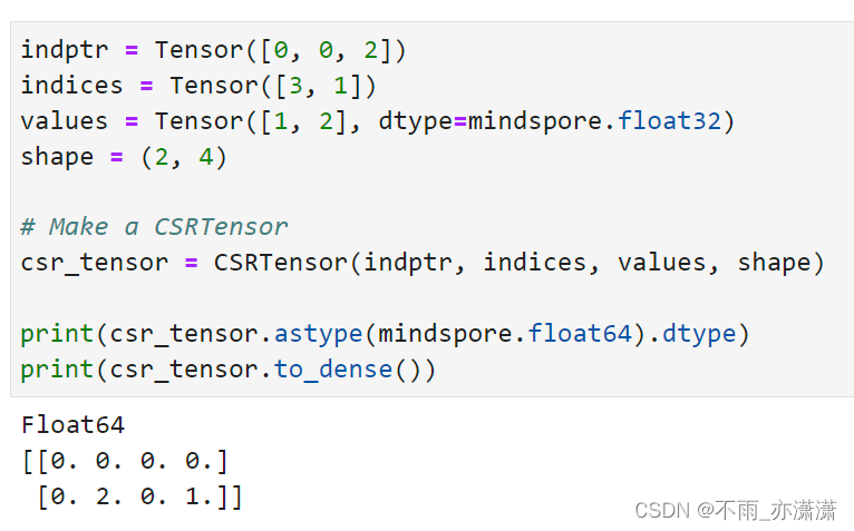

2️⃣ COOTensor
COO（Coordinate Format）稀疏张量格式用来表示某一张量在给定索引上非零元素的集合，若非零元素的个数为N，被压缩的张量的维数为ndims。各参数含义如下：

• indices: 二维整数张量，每行代表非零元素下标。形状：[N, ndims]， 索引数据类型支持int16、int32、int64。
• values: 一维张量，表示相对应的非零元素的值。形状：[N]。
• shape: 表示被压缩的稀疏张量的形状，目前仅支持二维COOTensor。

indices = Tensor([[0, 1], [1, 2]], dtype=mindspore.int32)
values = Tensor([1, 2], dtype=mindspore.float32)
shape = (3, 4)

# Make a COOTensor
coo_tensor = COOTensor(indices, values, shape)

print(coo_tensor.values)
print(coo_tensor.indices)
print(coo_tensor.shape)
print(coo_tensor.astype(mindspore.float64).dtype)  # COOTensor to float64

输出：

[1. 2.]
[[0 1]
 [1 2]]
(3, 4)
Float64

查看稠密形式：

print(coo_tensor.to_dense())

输出：

[[0. 1. 0. 0.]
 [0. 0. 2. 0.]
 [0. 0. 0. 0.]]

2. 小结

今天学习了Tensor，从如何创建到属性、运算、与Numpy互换，最后学习了稀疏张量。